Introduction To Python For Computational Science And Engineering

Fangohr, Hans. Introduction to Python for Computational Science and Engineering, 2015.

Fangohr’s book is an excellent introduction to python. Coming from a Matlab background, the structure is easy to follow and very useful. The only negative about this book is that it was written for Python 2 and I am working in 3. This generally didn’t pose any problems, mainly just remembering that in 3 print() requires brackets. My notes can be viewed as a Notebook on GitHub, of which some of the more interesting parts are included below.

General Notes

• Use help() with a command for details
• Use dir() with a command for a list of available methods

Chapter 2, A Powerful Calculator

import cmath

cmath.sqrt(-1)

1j

Chapter 5, Input and Output

• String specifiers, reprinted table below
• Pg 54-55 for a more elegant method of string formatting used in Python 3
• fileobject.readlines() method returns a list of strings

## Copied from Fangohr 2015, page 52.

AU = 149597870700  #Astronomical unit in [m]
"%g" %AU

'1.49598e+11'

hi

Chapter 8, Functional Tools

• Examples using the tools filter, reduce, and lamda.
• An anonymous function is only needed once or needs no name
  • lambda x : x**2
  • (lambda x, y, z: (x + y) * z)(10, 20, 2)
• The map function applies function f to all elements in sequence s, lst2 = map(f,s)
  • map(lambda x:x**2, range(10))
• The filter function applies the function f to all elements in a sequence s, lst2 = filter(f, lst)
  • The filet function should return a true or false.
  • filter(lambda x:x>5,range(11))
• List comprehension is an expression followed by a for clause, then zero or more for or if clauses. More consise then the above methods.

Chapter 12, Symbolic Computation

• SymPy is the Python Symbolic library, SymPy Homepage for full and up-to-date documentation
• Very slow compared to floating point opperation
• isympy an exexutable wrapper around python, convenient for figuring out new features or experementing interactively
• Rational type, Rational(1,2) represents 1/2.
  • Rational class works exactly as opposed to the standard float.
• If Sympy returns the result in an unfamiliar form, subtract it with the expected form to determine if they are equivalent.
• Calculate definite integrals with a tuple containing the variable of interest, lower, and upper bounds.
• Results from dsolve are an Equality class, function needs to be evaluated to a number to be plotted.
• preview() allows you to display rendered output on the screen
• Automatic generation of C code via codegen()

## Symbols

import sympy

x, y, z = sympy.symbols('x, y, z')

a = x + 2*y + 3*z - x

print(a)

print(sympy.sqrt(8))

2*y + 3*z
2*sqrt(2)

Differentiation

print(sympy.diff(3*x**4, x))
print(sympy.diff(3*x**4, x, x, x))
print(sympy.diff(3*x**4, x, 3))

12*x**3
72*x
72*x

Integration

from sympy import integrate

print(integrate(sympy.sin(x), y))
print(integrate(sympy.sin(x), x))

# Definite Integrals
print(integrate(x*2, x))
print(integrate(x*2, (x, 0, 2)))
print(integrate(x**2, (x,0,2), (x, 0, 2), (y,0,1)))

y*sin(x)
-cos(x)
x**2
4
16/3

Ordinary Differential Equations

from sympy import Symbol, dsolve, Function, Derivative, Eq

y = Function("y")
x = Symbol('x')
y_ = Derivative(y(x), x)
print(dsolve(y_ + 5*y(x), y(x)))
print(dsolve(Eq(y_ + 5*y(x), 0), y(x)))
print(dsolve(Eq(y_ + 5*y(x), 12), y(x)))

Eq(y(x), C1*exp(-5*x))
Eq(y(x), C1*exp(-5*x))
Eq(y(x), C1*exp(-5*x)/5 + 12/5)

Solving Non Linear Equations

import sympy

x, y, z = sympy.symbols('x,y,z')
eq = x - x**2
print(sympy.solve(eq,x))

[0, 1]

Chapter 15, Numerical Python (numpy): arrays

• The data structure, array, allows efficient matrix and vector operation
• An array can only keep elements of the same type, as opposed to lists which can hold a mix.
• Convert a matrix back tp a list or tuple using, list(s) or tuple(s).
• Computing eiganvectors and eiganvalues
• Numpy examples at SciPy.org

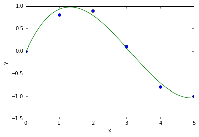
## Curve Fitting of Polynomial Example

import numpy

# demo curve fitting: xdata and ydata are input data
xdata = numpy.array([0.0, 1.0, 2.0, 3.0, 4.0, 5.0])
ydata = numpy.array([0.0, 0.8, 0.9, 0.1, -0.8, -1.0])

#now fit for cubic (order = 3) polynomial
z = numpy.polyfit(xdata, ydata, 3)

#z is an array of coefficients, highest first, i.e.
#          x^3         X^2      X       0
#z=array([0.08703704, -0.8134, 1.693, -0.0396])

print("z = ", z)

#It is convenient to use `poly1d` objects for dealing with polynomials
p = numpy.poly1d(z)    #Creates a polynomial function p from coefficients and p can be evaluated for all x then.

print("p = ",p)

#Create a plot
xs = [0.1 * i for i in range(50)]
ys = [p(x) for x in xs]    # evaluates p(x) for all x in list xs

%matplotlib inline
import pylab
pylab.plot(xdata, ydata, 'o', label = 'data')
pylab.plot(xs, ys, label = 'fitted curve')
pylab.ylabel('y')
pylab.xlabel('x')
#pylab.savefig('polyfit.pdf')
pylab.show()

z =  [ 0.08703704 -0.81349206  1.69312169 -0.03968254]
p =           3          2
0.08704 x - 0.8135 x + 1.693 x - 0.03968