Forced Vibrations With Viscous Damping

06 Jan 2017 | vibration

Steinberg, Dave. Vibration Analysis for Electronic Equipment, 2nd ed., 1988, Section 2.9

Given a mass-spring-damper system with a harmonic force $P_0 cos(\Omega t)$ acting on the mass. The sum of the forces is given by

\[m{\ddot Y} + c{\dot Y} + KY = P_0 cos(\Omega t).\]

Assume a solution for the motion of the mass is of the form

\[Y = Y_0 cos(\Omega t - \theta).\]

Taking the derivatives of this

\[{\dot Y} = Y_0 \Omega sin(\theta - \Omega t),\] \[{\ddot Y} = -Y_0 \Omega^2 cos(\theta - \Omega t).\]

Solving for $Y_0$ as a function of $P_0$ yeilds

\[Y_0 = \frac {P_0}{[(K - m\Omega^2)^2 + c^2\Omega^2]^\frac{1}{2}}.\]

From Steinberg, “The instantaneous magnitude of the force experienced by the support is the sum of the spring foce and the damper force. These two forces have a 90 degrees phase angle between them, so the force becomes

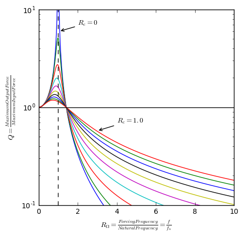
\[F_0 = Y_0(K^2 + c^2\Omega^2)^\frac{1}{2}."\]

Solving for $Y_0$ and plugging into the equation above yeilds an equation for $F_0$ as a function of $\Omega$ and cancels out $Y_0$. This can be used to solve for $Q = \frac{F_0}{P_0}$. Simplifying with $R_{\Omega}=\frac{\Omega}{\Omega_n}$ and $R_c=\frac{c}{c_c}$,

\[Q = \left[\frac{1 + (2R_{\Omega}R_c)^2}{(1-R_{\Omega}^2)^2 + (2R_{\Omega}R_c)^2}\right]^\frac{1}{2}\]

# Plotting Figure 2.17 using Eqn. 2.48.
%matplotlib inline
import matplotlib.pyplot as plt
from math import sqrt
import scipy as sp
from sympy import zeros
sp.seterr(divide='ignore')    # Ignore the 'divide by zero' error

R_c = sp.arange(0,1,.1)        # R_c = c/c_c. This is the ratio of the damping to the critical damping
R_Omega = sp.arange(0,10,.01)   # R_Omega = Omega / Omega_n.  This is the ratio of the input frequency to the natural frequency.

# Initialize the transmissibility Q 
Q = zeros(len(R_c), len(R_Omega))

# Equation 2.48
def Q_Rc_RO(R_Omega, R_c):
    Q = sqrt((1 + (2 * R_Omega * R_c)**2)/((1 - R_Omega**2)**2 + (2 * R_Omega * R_c)**2))
    return(Q)

for i in range(len(R_c)):
    for j in range(len(R_Omega)):
        Q[i,j] = Q_Rc_RO(R_Omega[j], R_c[i])
        
# Plot Results
plt.figure('Forced Vibration', figsize=[5,5])
plt.semilogy(R_Omega,Q.T)
plt.semilogy([1,1], [.1, 10], '--k')
plt.xlabel('$R_\Omega = \\frac{Forcing Frequency}{Natural Frequency} = \\frac{f}{f_n}$')
plt.ylabel('$Q = \\frac{Maximum Input Force}$')
plt.axis([0,10,0.1,10])
plt.plot([0,10],[1,1],'k')
plt.annotate(
    '$R_c = 0$', xy=(1.05,6), arrowprops=dict(arrowstyle='->'), xytext=(2,7))
plt.annotate(
    '$R_c = 1.0$', xy=(3,.575), arrowprops=dict(arrowstyle='->'), xytext=(4,.7))
plt.show()

png

Natural Design Exploring engineering boundaries.

Forced Vibrations With Viscous Damping