Outlive The Science And Art Of Longevity

Attia, Peter, and Bill Gifford. Outlive: The Science and Art of Longevity. Vermilion, 2023.

https://peterattiamd.com/outlive/

Summary

This book covers the cognative, physical, and emotional decline that occurs as we age. They then address steps we can take to minimize how far down this slope we shide using exercise, sleep, emotional heath, nutrition, and drugs. Attia and Gifford review in detail studies and the state of the art of each tactic cutting through the hyperbole common in reporting. Below I’ve caputred notes of interst to me as well as actions I can take to put these solutions into practice.

Workout and sleep more, eat and drink less. As we age our physical and cognative abilities degrade significantly from our current starting point. To improve our future capability we need to improve our starting position and continually work to combat the areas aging affects the most. We should strive to be at a peak of holistic performance while continuously monitoring our condition to address risks as early as possible.

Terms

• Mendelian Randomization ~ A tool to bridge long term trials using natural randomization.
• DNS ~ dynamic neuromuscular stabilization
• CR ~ Calorie restriction (calorie counting)
• DR ~ Dietary restrictions (diets)
• TR ~ Time restrictions (fasting)

Aging

• Centenarions not only live longer but they age better over time. Instead of focusing on individual fixes, a holistic method is required to reduce confounding factors.
• Autophagy is the cells process for cleaning our old matter. As we age this process decreases. Calorie restriction or Repamycin may improve autophagy.

What to Monitor

• Metabolic Syndrome, three of more of the following
  • Blood Pressure: > 130/85
  • Triglycerides: > 150 mg/dL
  • HDL chloresterol: < 40 mg/dL (<50 in women)
  • Waist circumference: > 40” (>35” in women)
  • Fasting glucose: > 110 mg/dL
• A dexa scan anually to track viscerol fat, body fat, and bone density.
• Colonoscopy at 40, repeated often depending on results.
  • Early detection is the best hope for reducing cancer mortality.
• apo B testing, heat disease precursur.
• Measure LDL, target < 20 mg/dL (hard to hit!)
• Lipid lower drugs (statins) should be considered early.
• Early signs of trouble
  • Increase in uric acid
  • Increase in homocysteine
  • Chronic inflamation
  • Increase in ALT liver enzymes

Cardio

• Zone 2 ~ A speed fast enough that a conversation becomes strained.
  • The maximum level of effort we can maintain without accumulating lactate.
  • With a lactate monitor: 1.7 - 2.0 millimoles
  • ~ 70 - 85% of peak heart rate
  • Three hours per week or four 45 minute sessions minimum
  • Two Watts per kilogram reasonable, shoot for 3 W/kg
• VO2 Max
  • Train for as high a V02 max as possible
  • Four mins (max pace you can sustain for four minutes), four minutes jogging, repeat four - six times.
  • Once per week unless training for an event

Strength

• Grip Strength
  • 60 second Farmers walk, 1/2 body weight in each hand
  • 120 second hang on pull up bar
• Pulling motions
  • Pull ups and Rows
• Eccentric strength
  • Down phase of pull ups, pull downs
  • Dead lifts, rows, downhill rucking
• Hip Hinging, high load
  • Single leg step ups, weights, video yourself to watch form.
  • Split stance RDLs

Stability

#1 Do yourself no harm!

• Work on stability 2 x per week, for 1 hour. 15 minutes other days.
• Attia Exercise Videos
• DNS, www.rehabps.com
• Good breathing
  • Chest, stomach, sides should expand evenly
  • Inhalation should be quiet, compared to breathing into your chest.
• Feet are the starting point for most activities
  • ‘toe yoga’
• One leg balance, eyes closed, > 10 seconds
• Use all four corners of your feet
• Slow cat-cow
  • Improve tech neck
  • Learn spinal segment control, feel each vertebre position.
• Shoulders, Scapular CARS
• Film to see what you are doing versus what you think you are doing.

Nutrition

• Protein when active. Its hard to eat too much protein, but it shoudl be split into multiple times during the day.
  • 1 gram / pound body weight / day
  • equal to: 1 oz / 30 lbs body weight, 0.1 lbs / 50 lbs body weight
  • Focus on Leucine, Lycine, and Methionine
  • 3 or 4 grams / day of leucine and lycine.
  • 1 gram / day of methionine
  • Increase lycine if trying to increase lean mass. 2/3 grams / serving, 4 x / day
  • Attia eats two meals with protein, has a protein snack, and a protein shake.
• Common paths. No one solution works for everyone. Often a combination is succesful.
  • CR ~ Calorie restriction (calorie counting)
  • DR ~ Dietary restrictions (diets)
  • TR ~ Time restrictions (fasting)
• Dont over drink, < 7 glasses / week and < 2 / day.
• Eat more olive oil, avacado, nuts, and salmon.
• EPA and DHA supplements
• Attia has ideal fat ratios for his patients, but it is determined on a patient by patient basis.
• Fasting
  • No clear benefits unless done deliberately for extreeme cases
  • Intermitant fasting barely works in the 8/16 ratio. This ratio makes it really difficult to get the protein required. It could be useful as a CR tool however.

Sleep

• Ashwagandha - potential sleep supplement
• Use a sleep tracker, but don’t stress the results.
• Good sleep environment
  • Remove all light sources. Dark curtains, no LEDs.
  • Warmer lights at night
  • Cold bed room, ~65 C

Forced Vibrations With Viscous Damping

Steinberg, Dave. Vibration Analysis for Electronic Equipment, 2nd ed., 1988, Section 2.9

Given a mass-spring-damper system with a harmonic force $P_0 cos(\Omega t)$ acting on the mass. The sum of the forces is given by

Assume a solution for the motion of the mass is of the form

Taking the derivatives of this

Solving for $Y_0$ as a function of $P_0$ yeilds

From Steinberg, “The instantaneous magnitude of the force experienced by the support is the sum of the spring foce and the damper force. These two forces have a 90 degrees phase angle between them, so the force becomes

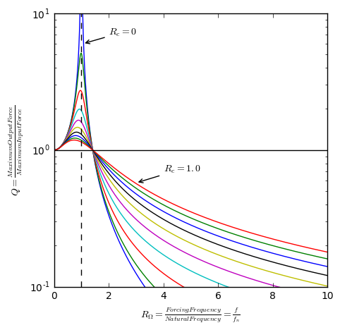
Solving for $Y_0$ and plugging into the equation above yeilds an equation for $F_0$ as a function of $\Omega$ and cancels out $Y_0$. This can be used to solve for $Q = \frac{F_0}{P_0}$. Simplifying with $R_{\Omega}=\frac{\Omega}{\Omega_n}$ and $R_c=\frac{c}{c_c}$,

# Plotting Figure 2.17 using Eqn. 2.48.
%matplotlib inline
import matplotlib.pyplot as plt
from math import sqrt
import scipy as sp
from sympy import zeros
sp.seterr(divide='ignore')    # Ignore the 'divide by zero' error

R_c = sp.arange(0,1,.1)        # R_c = c/c_c. This is the ratio of the damping to the critical damping
R_Omega = sp.arange(0,10,.01)   # R_Omega = Omega / Omega_n.  This is the ratio of the input frequency to the natural frequency.

# Initialize the transmissibility Q 
Q = zeros(len(R_c), len(R_Omega))

# Equation 2.48
def Q_Rc_RO(R_Omega, R_c):
    Q = sqrt((1 + (2 * R_Omega * R_c)**2)/((1 - R_Omega**2)**2 + (2 * R_Omega * R_c)**2))
    return(Q)

for i in range(len(R_c)):
    for j in range(len(R_Omega)):
        Q[i,j] = Q_Rc_RO(R_Omega[j], R_c[i])
        
# Plot Results
plt.figure('Forced Vibration', figsize=[5,5])
plt.semilogy(R_Omega,Q.T)
plt.semilogy([1,1], [.1, 10], '--k')
plt.xlabel('$R_\Omega = \\frac{Forcing Frequency}{Natural Frequency} = \\frac{f}{f_n}$')
plt.ylabel('$Q = \\frac{Maximum Input Force}$')
plt.axis([0,10,0.1,10])
plt.plot([0,10],[1,1],'k')
plt.annotate(
    '$R_c = 0$', xy=(1.05,6), arrowprops=dict(arrowstyle='->'), xytext=(2,7))
plt.annotate(
    '$R_c = 1.0$', xy=(3,.575), arrowprops=dict(arrowstyle='->'), xytext=(4,.7))
plt.show()

Vibration Analysis For Electronic Equipment

Steinberg, Dave. Vibration Analysis for Electronic Equipment, 2nd ed., 1988

Steinberg’s Vibration Analysis for Electric Equipment was recommended to me as a good text for improving my understanding of random vibration testing. This book turned out to be full of great information from the design of electronic chassis to fatigue analysis. Steinberg covers a large range of topics and starts with a simple model to explain each. Often, he will extend this analysis into a slightly more complex model, but with assumptions that simplify the model. I appreciate the detail with which the simple models were derived and would have liked to have seen similar detail in the second order systems.

I’ve taken notes on the areas related to my vibration work posted them to GitHub. Below is an excerpt of some of the interesting results.

Chapter 8, Understanding Random Vibration

• “If two major structural resonances occur close to one another, they may produce severe dynamic coupling effects that can produce rapid fatigue failures.”
• For a cyclically alternating electric current, RMS is equal to the value of the direct current that would produce the same average power dissipation in a resistive load.
• Failure conditions
  1. High acceleration levels
  2. High stress levels
  3. Large displacement amplitudes
  4. Electrical signals out of tolerance - N.A.
• $3\sigma$ is often the limit used because it captures 99.7% of the accelerations and most labs have a $3\sigma$ limit on their equipment.
• In the math library, natural log is called with (log) and log base 10 with (log10)
• Multiple degree of freedom systems (8.29). $G_{out} = \sqrt(\sum(P_i \Delta f_i Q_i^2))$
• From: Crandall, Random Vibration, 1958. $P_{out} = Q^2 P$. Book available online.

## Calculating the Grms of a shaped random vibration input curve.
# Sec. 8.8, Eqns. 8.4 - 8.6.

def grms (freq, PSD):
    """Returns the Grms value for a shaped random vibration input curve.
    Input the frequency and PSD values as a list in the form grms(freq, PSD).
    The frequency and PSD list must have the same number of elements."""
    
    from math import log10, log
    
    A = 0
    
    if len(freq)!=len(PSD):
        print("Error: The number of elements in the Frequency and PSD lists do not match.")
    
    else:
        for i in range(1,len(freq)):
            
            # Calculate the slope
            dB = 10 * log10(PSD[i]/PSD[i-1])           # dB
            OCT = log10(freq[i]/freq[i-1])/log10(2)    # Octave
            S = dB/OCT                                 # Slope
            
            # Calculate the area in units of [G^2]
            if S == 0:
                A = A + PSD[i] * (freq[i] - freq[i-1])
            elif S == -3:
                A = A + -freq[i] * PSD[i] * log(freq[i-1] / freq[i])
            else:
                A = A + (3 * PSD[i]/(3 + S)) * (freq[i] - (freq[i-1]/freq[i])**(S/3) * freq[i-1])
            
            # Calculate the Grms [G]
            grms = A**(0.5)

    return(grms)

# Find the GRMS of the ASTM common carrier profile.  

Common_Carrier = [[1, 4, 100, 200], [.0001, .01, .01, .001]]

grms(Common_Carrier[0], Common_Carrier[1])

1.1469379669303117

## Response to a random vibration, from Section 8.
# Valid for a single resonance with a Q > 10.


def resp_psd_Q (P_in, Q, f_n, g=9800):
    """At a natural frequency, calculates the Grms and Zrms (relative motion) of the point given the transmissibility,
    and PSD.""" 
    from math import pi
    
    Grms = ((pi/2)*P_in*f_n*Q)**0.5    # RMS acceleration, Eqn. 8.61
    
    #g = 9.8*1000                       # Gravity, [mm/s^2]
    
    Zrms = Y_G_fn(Grms, f_n, g)      # Relative motion, Eqn. 8.62.  Ref. Eqn. 2.30
    
    return(Grms, Zrms)

resp_psd_Q (0.00072, 3.146, 30.4)

(0.3288836909042307, 0.08834083693899289)

Chapter 9, Designing for Shock Environments

• Eqn. 9.40 - Damping ratio ~ $R_c = \frac{C}{C_c} = \frac{1}{2 Q}$ \(Q = \frac{1}{2 R_c}\)
• Figure 9.17 illustrates the difficulty in designing for both shock and vibration. Shock isolation occurs to the left of the amplification peak while vibration isolation occurs on the right. Equation for calculating amplification missing for graphs in Chp. 9.
• Velocity shocks, used when modeling drop tests.
  • Assuming single DOF M-S-D, the dork done on the spring is equal to the kinetic energy of the mass. $\frac{1}{2} K Y^2 = \frac{1}{2} M V^2$
  • Max acceleration: $G_{max} = \frac{a}{g} = \frac{V}{g} \sqrt(\frac{K}{M}) = \frac{V}{g} \Omega$, or $G = \frac{\Delta V \Omega}{g}$.
• Can not recreate Fig. 9.21 without a relationship between the amplification and the frequency ratio.
  • Impact damping only occurs at $R = \frac{f_{response}}{f_{source}} <= 0.5$
  • Danger area from $0.5 <= R <= 2$
  • This assumes an damping ratio of $R_c = 0.1$ and $Q = 5$.
  • These equations do not relate to velocity shocks in which the forcing frequency is determined by the natural frequency.
• For velocity shocks max expected G can be calculated or if the response is known, the natural frequency should fall out as function of the response G and the height.

# Calculate the velocity before impact during drop tests
def vf_H (H, g=9800):
    '''Solves for the velocity before impact of an object dropped from a height H.
    Assumes a standard gravity of 9800 mm/s. Input the gravity in the same unit system as the height.'''
    
    v = (2*g*H)**0.5
    
    return v

# For a 2" drop
vf = vf_H(2*2.54)
print(vf)

315.54397474837003

# Find G_max due to a drop test

def gmax_drop (H, fn, g=9800):
    '''Find the maximum acceleration due to a velocity shock given the drop height (H), 
    natural frequency (fn), and gravity (g). The gravity should be input in the same
    unit system as the velocity.  Defaults to mm/s^2
    
    Returns max acceleration in Gs (unitless)'''
    
    from math import pi
    
    v = (2*g*H)**0.5
    g_max = v*(2*pi*fn)/g
    
    return(g_max)

def fn_drop (H, g_max, g=9800):
    '''Find the natural frequency of a system based on a  shock
    from a given the height (H), maximum acceleration response (g_max), 
    and gravity (g). The gravity should be input in the same
    unit system as the velocity.  Defaults to mm/s^2
    
    Returns natural freuqncy f_n [Hz]'''
    
    from math import pi
    
    v = (2*g*H)**0.5
    fn = g_max*g/(v*2*pi)
    
    return(fn)

H = 2       #[in]
H = H*25.4  #[mm]

g_max = gmax_drop(H, 14)
fn = fn_drop(H, 10)

print('Max G: ', g_max)
print('Natural Frequency: ', fn)

Max G:  8.95656991107948
Natural Frequency:  15.630983891145293

Introduction To Python For Computational Science And Engineering

Fangohr, Hans. Introduction to Python for Computational Science and Engineering, 2015.

Fangohr’s book is an excellent introduction to python. Coming from a Matlab background, the structure is easy to follow and very useful. The only negative about this book is that it was written for Python 2 and I am working in 3. This generally didn’t pose any problems, mainly just remembering that in 3 print() requires brackets. My notes can be viewed as a Notebook on GitHub, of which some of the more interesting parts are included below.

General Notes

• Use help() with a command for details
• Use dir() with a command for a list of available methods

Chapter 2, A Powerful Calculator

import cmath

cmath.sqrt(-1)

1j

Chapter 5, Input and Output

• String specifiers, reprinted table below
• Pg 54-55 for a more elegant method of string formatting used in Python 3
• fileobject.readlines() method returns a list of strings

## Copied from Fangohr 2015, page 52.

AU = 149597870700  #Astronomical unit in [m]
"%g" %AU

'1.49598e+11'

hi

Chapter 8, Functional Tools

• Examples using the tools filter, reduce, and lamda.
• An anonymous function is only needed once or needs no name
  • lambda x : x**2
  • (lambda x, y, z: (x + y) * z)(10, 20, 2)
• The map function applies function f to all elements in sequence s, lst2 = map(f,s)
  • map(lambda x:x**2, range(10))
• The filter function applies the function f to all elements in a sequence s, lst2 = filter(f, lst)
  • The filet function should return a true or false.
  • filter(lambda x:x>5,range(11))
• List comprehension is an expression followed by a for clause, then zero or more for or if clauses. More consise then the above methods.

Chapter 12, Symbolic Computation

• SymPy is the Python Symbolic library, SymPy Homepage for full and up-to-date documentation
• Very slow compared to floating point opperation
• isympy an exexutable wrapper around python, convenient for figuring out new features or experementing interactively
• Rational type, Rational(1,2) represents 1/2.
  • Rational class works exactly as opposed to the standard float.
• If Sympy returns the result in an unfamiliar form, subtract it with the expected form to determine if they are equivalent.
• Calculate definite integrals with a tuple containing the variable of interest, lower, and upper bounds.
• Results from dsolve are an Equality class, function needs to be evaluated to a number to be plotted.
• preview() allows you to display rendered output on the screen
• Automatic generation of C code via codegen()

## Symbols

import sympy

x, y, z = sympy.symbols('x, y, z')

a = x + 2*y + 3*z - x

print(a)

print(sympy.sqrt(8))

2*y + 3*z
2*sqrt(2)

Differentiation

print(sympy.diff(3*x**4, x))
print(sympy.diff(3*x**4, x, x, x))
print(sympy.diff(3*x**4, x, 3))

12*x**3
72*x
72*x

Integration

from sympy import integrate

print(integrate(sympy.sin(x), y))
print(integrate(sympy.sin(x), x))

# Definite Integrals
print(integrate(x*2, x))
print(integrate(x*2, (x, 0, 2)))
print(integrate(x**2, (x,0,2), (x, 0, 2), (y,0,1)))

y*sin(x)
-cos(x)
x**2
4
16/3

Ordinary Differential Equations

from sympy import Symbol, dsolve, Function, Derivative, Eq

y = Function("y")
x = Symbol('x')
y_ = Derivative(y(x), x)
print(dsolve(y_ + 5*y(x), y(x)))
print(dsolve(Eq(y_ + 5*y(x), 0), y(x)))
print(dsolve(Eq(y_ + 5*y(x), 12), y(x)))

Eq(y(x), C1*exp(-5*x))
Eq(y(x), C1*exp(-5*x))
Eq(y(x), C1*exp(-5*x)/5 + 12/5)

Solving Non Linear Equations

import sympy

x, y, z = sympy.symbols('x,y,z')
eq = x - x**2
print(sympy.solve(eq,x))

[0, 1]

Chapter 15, Numerical Python (numpy): arrays

• The data structure, array, allows efficient matrix and vector operation
• An array can only keep elements of the same type, as opposed to lists which can hold a mix.
• Convert a matrix back tp a list or tuple using, list(s) or tuple(s).
• Computing eiganvectors and eiganvalues
• Numpy examples at SciPy.org

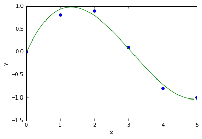
## Curve Fitting of Polynomial Example

import numpy

# demo curve fitting: xdata and ydata are input data
xdata = numpy.array([0.0, 1.0, 2.0, 3.0, 4.0, 5.0])
ydata = numpy.array([0.0, 0.8, 0.9, 0.1, -0.8, -1.0])

#now fit for cubic (order = 3) polynomial
z = numpy.polyfit(xdata, ydata, 3)

#z is an array of coefficients, highest first, i.e.
#          x^3         X^2      X       0
#z=array([0.08703704, -0.8134, 1.693, -0.0396])

print("z = ", z)

#It is convenient to use `poly1d` objects for dealing with polynomials
p = numpy.poly1d(z)    #Creates a polynomial function p from coefficients and p can be evaluated for all x then.

print("p = ",p)

#Create a plot
xs = [0.1 * i for i in range(50)]
ys = [p(x) for x in xs]    # evaluates p(x) for all x in list xs

%matplotlib inline
import pylab
pylab.plot(xdata, ydata, 'o', label = 'data')
pylab.plot(xs, ys, label = 'fitted curve')
pylab.ylabel('y')
pylab.xlabel('x')
#pylab.savefig('polyfit.pdf')
pylab.show()

z =  [ 0.08703704 -0.81349206  1.69312169 -0.03968254]
p =           3          2
0.08704 x - 0.8135 x + 1.693 x - 0.03968

Creating a GitHub Blog and Sharing Jupyter Notebooks

This blog was hacked together using a lot of different examples which I’ve attempted to detail below. This was built with a Windows machine using:

• Anaconda
• GitHub Desktop
• MarkdownPad 2

All of the files for this blog can be found on my GitHub.

Goals

I had the following goals in mind while trying to piece together this blog.

• Static blog using GitHub Pages
• Clean and modern looking interface
• Easy to write, edit, and upload posts
• Ability to include Jupyter notebooks easily
• Search-able post tags

Method

A list of the sites, blogs, and github directories that I used to create this site. This is not meant to be an instruction manual for creating a similar blog, but it should get you started.

Getting Started

• I started with the GitHub pages tutorial.
• The majority of my blog was then forked from Bruce Eckel’s GitHub page following his tutorial in Using Github Pages for Blogging
  • I needed to install easygui.py to get the newpost.bat program to work.
  • I made a few minor style tweaks I’ll try to detail below.
  • I added tag and jupyter functionality.
• I used this post Build A Blog With Jekyll And GitHub Pages and the fork above to get the site up and running.
• To add Jupyter notebooks I followed the steps on Brian Caffey’s post, Including Jupyter Notebooks in Jekyll blog posts.
  • I recommend adding the image files to a new folder with the path /public/img/.
  • I need to create a python script to automate the path insertion. [To-Do]
• Finally, I wanted my posts to be organized with tags. I used the method detailed in Use Tags and Categories in your Jekyll based Github Pages without plugins.
  • This required a bit of tweaking to make it work with the basic site. I added the category.html and tag.html to the base folder with index.html.
  • I changed the title of each to Categories and Tags and layout to default for both.
  • I added Tags and Categories to the header.
  • For the links on the Category and Tag pages, I needed to use <code> instead of <small>.
  • Finally, I commented out the header used in the index to minimize clutter on the front page.
  • I need to modify the newpost.bat to include tags and categories. [To-Do]
  • I would like to add icons for categories, tags, email, linked, and github. [To-Do]

Tips and Tricks

• The theme can be modified by changing the body class in the default.html. Available themes and other options can be found on the Lanyon GitHub page.
• I modified my sidebar to use a table for the links at the top as opposed to the original simple list. This let me keep them centered.
  • I needed to pull the theme background color from the index and input it into the <td> field to overwrite the existing table highlighting. This breaks the ability to add a hover feature to <td>.
• I referenced this site often when tweaking my tables in the sidebar.
• I used Powerpoint to create my simple favicon (website icon). Then I used the online Favicon & App Icon Generator and Favicon Generator. For real.. The first generator creates more icons and the second gives you more control over how the icons will look on mobile devices. Both sites was simple and easy to use. Take these images and extract them to your /public/icon/ path. Update your head.html file to include the icon locations as detailed by the generator sites. Make sure to update the generic locations with public/icon. Open public/icon/manifest.json and add you name as it should be displayed on a mobile device, "name": "Site Name Here". Finally, add the browserconfig.xml to the root directory. It took a while for the old favicon to be replaced by the new one, try checking with a different web browser or clearing your cache.
• For troubleshooting elements of the blog, I would make small changes and commit them. Then I would open the website in incognito mode to prevent my browser from storing any of the data. This allowed me to check features pretty quickly.
  • Be careful when modifying the header of posts. Adding returns seems to break the post.
• I ran into a lot of problems trying to display the HTML code within this post. Many of the methods I tried ended up breaking the post causing it to not display. I would then receive an email from GitHub with “The value ‘nil’ was passed to a date-related filter that expects valid dates…”. The solution I used was to submit Gists and embed the generated <script src=... code.
• To make the code look nice and add some style to the Tag and Category pages I used <code class="highlighter-rouge">...</code>. Adding the code block inside <a href>...</a> results in a different color than adding it to the outside. I used this to differentiate between the tags and the dates.
• I thought it would be fun to convert my resume to markdown and included it in the sidebar. I used the example detailed in blm.io’s Building an academic CV in markdown.
• A reference I have up constantly is daringfireball.net’s Markdown: Syntax.
• A tool that generates color pallets at ColorHexa.